GIS mapping in R
Marie-Hélène Burle
February 3, 2021

Great resources
Open GIS data
Free GIS Data
: list of free GIS datasets
Books
Geocomputation with R
by Robin Lovelace, Jakub Nowosad & Jannes Muenchow
Spatial Data Science
by Edzer Pebesma & Roger Bivand
Spatial Data Science with R
by Robert J. Hijmans
Using Spatial Data with R
by Claudia A. Engel
Tutorial
An Introduction to Spatial Data Analysis and Visualisation in R
by the CDRC
Website
r-spatial
by Edzer Pebesma, Marius Appel & Daniel Nüst
CRAN package list
Analysis of Spatial Data
Mailing list
R Special Interest Group on using Geographical data and Mapping
Data
For this webinar, we will use:
- the Alaska as well as the Western Canada & USA subsets of the Randolph Glacier Inventory version 6.01
- the USGS time series of the named glaciers of Glacier National Park 2
- the Alaska as well as the Western Canada & USA subsets of the consensus estimate for the ice thickness distribution of all glaciers on Earth dataset 3
The datasets can be downloaded as zip files from these websites.
-
RGI Consortium (2017). Randolph Glacier Inventory – A Dataset of Global Glacier Outlines: Version 6.0: Technical Report, Global Land Ice Measurements from Space, Colorado, USA. Digital Media. DOI: https://doi.org/10.7265/N5-RGI-60.
-
Fagre, D.B., McKeon, L.A., Dick, K.A. & Fountain, A.G., 2017, Glacier margin time series (1966, 1998, 2005, 2015) of the named glaciers of Glacier National Park, MT, USA: U.S. Geological Survey data release. DOI: https://doi.org/10.5066/F7P26WB1.
-
Farinotti, Daniel, 2019, A consensus estimate for the ice thickness distribution of all glaciers on Earth - dataset, Zurich. ETH Zurich. DOI: https://doi.org/10.3929/ethz-b-000315707.
Basemap
We will use data from Natural Earth
, a public domain map dataset.
This dataset can be accessed direction from within R thanks to the packages rnaturalearth (provides the functions) & rnaturalearthdata (provides the data).
Load packages
library(sf)                 # spatial vector data manipulation
library(tmap)               # map production & tiled web map
library(dplyr)              # non GIS specific (tabular data manipulation)
library(magrittr)           # non GIS specific (pipes)
library(purrr)              # non GIS specific (functional programming)
library(rnaturalearth)      # basemap data access functions
library(rnaturalearthdata)  # basemap data
library(mapview)            # tiled web map
library(grid)               # (part of base R) used to create inset map
library(ggmap)              # download basemap data
library(basemaps)           # download basemap data
library(ggplot2)            # alternative to tmap for map production
library(raster) # gridded spatial data manipulationNote on installing packages
Packages on CRAN can be installed with:
install.packages("<package-name>")
basemaps is not on CRAN and needs to be installed from GitHub thanks to devtools:
install.packages("devtools")
devtools::install_github("16EAGLE/basemaps")
sf
Great package for spatial vector data
Reading in data
Download and unzip 02_rgi60_WesternCanadaUS & 01_rgi60_Alaska from the Randolph Glacier Inventory
version 6.0.
Data get imported and turned into sf objects with the function sf::st_read():
ak <- st_read("01_rgi60_Alaska")
wes <- st_read("02_rgi60_WesternCanadaUS")Reading in data
> Reading layer '01_rgi60_Alaska' using driver 'ESRI Shapefile'
Simple feature collection with 27108 features and 22 fields
geometry type:  POLYGON
dimension:      XY
bbox:           xmin: -176.1425 ymin: 52.05727 xmax: -126.8545 ymax: 69.35167
geographic CRS: WGS 84
> Reading layer '02_rgi60_WesternCanadaUS' using driver 'ESRI Shapefile'
Simple feature collection with 18855 features and 22 fields
geometry type:  MULTIPOLYGON
dimension:      XY
bbox:           xmin: -133.7324 ymin: 36.38625 xmax: -105.6082 ymax: 65.15664
geographic CRS: WGS 84
First look at the data
> ak
Simple feature collection with 27108 features and 22 fields
geometry type:  POLYGON
dimension:      XY
bbox:           xmin: -176.1425 ymin: 52.05727 xmax: -126.8545 ymax: 69.35167
geographic CRS: WGS 84
First 10 features:
		   RGIId        GLIMSId  BgnDate  EndDate    CenLon   CenLat O1Region
1  RGI60-01.00001 G213177E63689N 20090703 -9999999 -146.8230 63.68900        1
2  RGI60-01.00002 G213332E63404N 20090703 -9999999 -146.6680 63.40400        1
3  RGI60-01.00003 G213920E63376N 20090703 -9999999 -146.0800 63.37600        1
4  RGI60-01.00004 G213880E63381N 20090703 -9999999 -146.1200 63.38100        1
5  RGI60-01.00005 G212943E63551N 20090703 -9999999 -147.0570 63.55100        1
6  RGI60-01.00006 G213756E63571N 20090703 -9999999 -146.2440 63.57100        1
7  RGI60-01.00007 G213771E63551N 20090703 -9999999 -146.2295 63.55085        1
8  RGI60-01.00008 G213704E63543N 20090703 -9999999 -146.2960 63.54300        1
9  RGI60-01.00009 G212400E63659N 20090703 -9999999 -147.6000 63.65900        1
10 RGI60-01.00010 G212830E63513N 20090703 -9999999 -147.1700 63.51300        1
O2Region   Area Zmin Zmax Zmed Slope Aspect  Lmax Status Connect Form
1         2  0.360 1936 2725 2385    42    346   839      0       0    0
2         2  0.558 1713 2144 2005    16    162  1197      0       0    0
3         2  1.685 1609 2182 1868    18    175  2106      0       0    0
4         2  3.681 1273 2317 1944    19    195  4175      0       0    0
5         2  2.573 1494 2317 1914    16    181  2981      0       0    0
6         2 10.470 1201 3547 1740    22     33 10518      0       0    0
7         2  0.649 1918 2811 2194    23    151  1818      0       0    0
8         2  0.200 2826 3555 3195    45     80   613      0       0    0
9         2  1.517 1750 2514 1977    18    274  2255      0       0    0
10        2  3.806 1280 1998 1666    17     35  3332      0       0    0
TermType Surging Linkages Name                       geometry
1         0       9        9 <NA> POLYGON ((-146.818 63.69081...
2         0       9        9 <NA> POLYGON ((-146.6635 63.4076...
3         0       9        9 <NA> POLYGON ((-146.0723 63.3834...
4         0       9        9 <NA> POLYGON ((-146.149 63.37919...
5         0       9        9 <NA> POLYGON ((-147.0431 63.5502...
6         0       9        9 <NA> POLYGON ((-146.2436 63.5562...
7         0       9        9 <NA> POLYGON ((-146.2495 63.5531...
8         0       9        9 <NA> POLYGON ((-146.2992 63.5443...
9         0       9        9 <NA> POLYGON ((-147.6147 63.6643...
10        0       9        9 <NA> POLYGON ((-147.1494 63.5098...
Structure of the data
> str(ak)
Classes ‘sf’ and 'data.frame':	27108 obs. of  23 variables:
$ RGIId   : chr  "RGI60-01.00001" "RGI60-01.00002" "RGI60-01.00003"  ...
$ GLIMSId : chr  "G213177E63689N" "G213332E63404N" "G213920E63376N" ...
$ BgnDate : chr  "20090703" "20090703" "20090703" "20090703" ...
$ EndDate : chr  "-9999999" "-9999999" "-9999999" "-9999999" ...
$ CenLon  : num  -147 -147 -146 -146 -147 ...
$ CenLat  : num  63.7 63.4 63.4 63.4 63.6 ...
$ O1Region: chr  "1" "1" "1" "1" ...
$ O2Region: chr  "2" "2" "2" "2" ...
$ Area    : num  0.36 0.558 1.685 3.681 2.573 ...
$ Zmin    : int  1936 1713 1609 1273 1494 1201 1918 2826 1750 1280 ...
$ Zmax    : int  2725 2144 2182 2317 2317 3547 2811 3555 2514 1998 ...
$ Zmed    : int  2385 2005 1868 1944 1914 1740 2194 3195 1977 1666 ...
$ Slope   : num  42 16 18 19 16 22 23 45 18 17 ...
$ Aspect  : int  346 162 175 195 181 33 151 80 274 35 ...
$ Lmax    : int  839 1197 2106 4175 2981 10518 1818 613 2255 3332 ...
$ Status  : int  0 0 0 0 0 0 0 0 0 0 ...
$ Connect : int  0 0 0 0 0 0 0 0 0 0 ...
$ Form    : int  0 0 0 0 0 0 0 0 0 0 ...
$ TermType: int  0 0 0 0 0 0 0 0 0 0 ...
$ Surging : int  9 9 9 9 9 9 9 9 9 9 ...
$ Linkages: int  9 9 9 9 9 9 9 9 9 9 ...
$ Name    : chr  NA NA NA NA ...
$ geometry:sfc_POLYGON of length 27108; first list element: List of 1
..$ : num [1:65, 1:2] -147 -147 -147 -147 -147 ...
..- attr(*, "class")= chr [1:3] "XY" "POLYGON" "sfg"
- attr(*, "sf_column")= chr "geometry"
- attr(*, "agr")= Factor w/ 3 levels "constant","aggregate",..: NA NA NA NA ...
..- attr(*, "names")= chr [1:22] "RGIId" "GLIMSId" "BgnDate" "EndDate" ...
Mapping with tmap
Combining datasets
> st_crs(ak) == st_crs(wes)
[1] TRUE
The spatial bounding boxes (bbox) however are different
(of course, since the 2 datasets cover different geographic areas)
> st_bbox(ak) == st_bbox(wes)
 xmin  ymin  xmax  ymax
FALSE FALSE FALSE FALSE
Union of bounding boxes
nwa_bbox <- st_bbox(
  st_union(
	st_as_sfc(st_bbox(wes)),
	st_as_sfc(st_bbox(ak))
  )
)
Our new bounding box for the map of Western North America:
> nwa_bbox
	  xmin       ymin       xmax       ymax
-176.14247   36.38625 -105.60821   69.35167
Glaciers of Western North America
tm_shape(ak, bbox = nwa_bbox) +
  tm_polygons() +
  tm_shape(wes) +
  tm_polygons() +
  tm_layout(
	title = "Glaciers of Western North America",
	title.position = c("center", "top"),
	title.size = 1.1,
	bg.color = "#fcfcfc",
	inner.margins = c(0.06, 0.01, 0.09, 0.01),
	outer.margins = 0,
	frame.lwd = 0.2
  ) +
  tm_compass(
	type = "arrow",
	position = c("right", "top"),
	size = 1.2,
	text.size = 0.6
  ) +
  tm_scale_bar(
	breaks = c(0, 1000, 2000),
	position = c("right", "BOTTOM")
  )
Basemaps
Let’s add one to our map of the glaciers of WNA
Getting a basemap from rnaturalearth
states_all <- ne_states(
  country = c("canada", "united states of america"),
  returnclass = "sf"
)
Selection of relevant states/provinces
states <- states_all %>%
  filter(name_en == "Alaska" |
		   name_en == "British Columbia" |
		   name_en == "Yukon" |
		   name_en == "Northwest Territories" |
		   name_en ==  "Alberta" |
		   name_en == "California" |
		   name_en == "Washington" |
		   name_en == "Oregon" |
		   name_en == "Idaho" |
		   name_en == "Montana" |
		   name_en == "Wyoming" |
		   name_en == "Colorado" |
		   name_en == "Nevada" |
		   name_en == "Utah"
		 )
Adding a basemap to our map: a few notes
Always make sure the CRS match!
> st_crs(states) == st_crs(ak)
[1] TRUE
The bounding boxes are different and we are only interested in the basemap within the bounding box of our data, so this is the only part of the basemap that we will plot.
> st_bbox(states) == nwa_bbox
xmin  ymin  xmax  ymax
FALSE FALSE FALSE FALSE
Play with colors of borders and fill, as well as the width of the borders.
Add the basemap to our map
tm_shape(states, bbox = nwa_bbox) +
  tm_polygons(col = "#f2f2f2",
			  lwd = 0.2) +
  tm_shape(ak) +
  tm_borders(col = "#3399ff") +
  tm_fill(col = "#86baff") +
  tm_shape(wes) +
  tm_borders(col = "#3399ff") +
  tm_fill(col = "#86baff") +
  tm_layout(
	title = "Glaciers of Western North America",
	title.position = c("center", "top"),
	title.size = 1.1,
	bg.color = "#fcfcfc",
	inner.margins = c(0.06, 0.01, 0.09, 0.01),
	outer.margins = 0,
	frame.lwd = 0.2
  ) +
  tm_compass(
	type = "arrow",
	position = c("right", "top"),
	size = 1.2,
	text.size = 0.6
  ) +
  tm_scale_bar(
	breaks = c(0, 1000, 2000),
	position = c("right", "BOTTOM")
  )
Maps based on an attribute variable
Retreat of glaciers over time
in Glacier National Park
We will use the USGS time series of the named glaciers of Glacier National Park
.
These 4 datasets have the contour lines of 39 glaciers for the years 1966, 1998, 2005, and 2015.
Cleaning datasets
## create a function that reads and cleans the data
prep <- function(dir) {
  g <- st_read(dir)
  g %<>% rename_with(~ tolower(gsub("Area....", "area", .x)))
  g %<>% dplyr::select(
	year,
	objectid,
	glacname,
	area,
	shape_leng,
	x_coord,
	y_coord,
	source_sca,
	source
  )
}

## create a vector of dataset names
dirs <- grep("GNPglaciers_.*", list.dirs(), value = T)

## pass each element of that vector through prep() thanks to map()
gnp <- map(dirs, prep)Combining datasets into one sf object
Checking that the CRS are the same:
> st_crs(gnp[[1]]) == st_crs(gnp[[2]])
[1] TRUE
> st_crs(gnp[[1]]) == st_crs(gnp[[3]])
[1] TRUE
> st_crs(gnp[[1]]) == st_crs(gnp[[4]])
[1] TRUE
We can rbind our lists:
gnp <- do.call("rbind", gnp)The Glacier National Park data
> gnp
Simple feature collection with 156 features and 9 fields
geometry type:  MULTIPOLYGON
dimension:      XY
bbox:           xmin: 263221.4 ymin: 5355550 xmax: 314490 ymax: 5430612
projected CRS:  NAD83 / UTM zone 12N
First 10 features:
   year objectid          glacname       area shape_leng          x_coord
1  1966        1   Agassiz Glacier 1600559.73 15177.8599 268743.351899585
2  1966        2     Ahern Glacier  589185.63  3435.4477 295758.255307284
3  1966        3      Baby Glacier  117171.13  1615.1598 268883.636523344
4  1966        4 Blackfoot Glacier 1832451.35 13980.9680 303273.800396565
5  1966        5   Boulder Glacier  231017.73  2847.2854 273967.708607631
6  1966        6    Carter Glacier  355743.44  3797.6787 276453.100195484
7  1966        7    Chaney Glacier  563819.03  4574.1331 292401.981825031
8  1966        8     Dixon Glacier  291142.05  4290.1178 279133.259744622
9  1966        9       Gem Glacier   29140.12   729.2132 299428.059935107
10 1966       10     Grant Glacier  347753.17  3566.9214 296042.327952401
			y_coord source_sca                                           source
1  5424909.85602688    1:24000        USGS 7.5 minute quadrangle map, 1966-1968
2  5413721.34271866    1:24000        USGS 7.5 minute quadrangle map, 1966-1968
3  5421759.44177687    1:24000        USGS 7.5 minute quadrangle map, 1966-1968
4  5385742.56009277    1:24000        USGS 7.5 minute quadrangle map, 1966-1968
5  5427330.78714926    1:24000        USGS 7.5 minute quadrangle map, 1966-1968
6  5419732.76738801    1:24000  USGS 7.5 minute quadrangle map, 66-68/NAIP 2005
7  5414857.32230536    1:24000        USGS 7.5 minute quadrangle map, 1966-1968
8  5423939.24915264    1:24000        USGS 7.5 minute quadrangle map, 1966-1968
9  5402885.93646811    1:24000 USGS Orthorectified Aerial Image from 08/24/1966
10  5356015.8412555    1:24000        USGS 7.5 minute quadrangle map, 1966-1968
						 geometry
1  MULTIPOLYGON (((269058 5425...
2  MULTIPOLYGON (((296217 5413...
3  MULTIPOLYGON (((269177.9 54...
4  MULTIPOLYGON (((304232.1 53...
5  MULTIPOLYGON (((274147.3 54...
6  MULTIPOLYGON (((276305.8 54...
7  MULTIPOLYGON (((291893.1 54...
8  MULTIPOLYGON (((279083.7 54...
9  MULTIPOLYGON (((299492.6 54...
10 MULTIPOLYGON (((295555.1 53...
Structure of Glacier National Park data
> str(gnp)
Classes ‘sf’ and 'data.frame':	156 obs. of  10 variables:
$ year      : chr  "1966" "1966" "1966" "1966" ...
$ objectid  : num  1 2 3 4 5 6 7 8 9 10 ...
$ glacname  : chr  "Agassiz Glacier" "Ahern Glacier" "Baby Glacier" ...
$ area      : num  1600560 589186 117171 1832451 231018 ...
$ shape_leng: num  15178 3435 1615 13981 2847 ...
$ x_coord   : chr  "268743.351899585" "295758.255307284" ...
$ y_coord   : chr  "5424909.85602688" "5413721.34271866" ...
$ source_sca: chr  "1:24000" "1:24000" "1:24000" "1:24000" ...
$ source    : chr  "USGS 7.5 minute quadrangle map, 1966-1968" ...
$ geometry  :sfc_MULTIPOLYGON of length 156; first list element: List of 1
..$ :List of 12
.. ..$ : num [1:214, 1:2] 269058 269075 269117 269165 269205 ...
.. ..$ : num [1:14, 1:2] 268591 268591 268603 268620 268630 ...
.. ..$ : num [1:9, 1:2] 268658 268692 268723 268726 268737 ...
.. ..$ : num [1:10, 1:2] 269256 269234 269239 269272 269348 ...
.. ..$ : num [1:10, 1:2] 268996 269003 269049 269154 269163 ...
.. ..$ : num [1:19, 1:2] 269402 269470 269486 269487 269509 ...
.. ..$ : num [1:10, 1:2] 269084 269122 269141 269152 269116 ...
.. ..$ : num [1:12, 1:2] 269464 269487 269559 269580 269576 ...
.. ..$ : num [1:8, 1:2] 268893 268923 268939 268925 268884 ...
.. ..$ : num [1:9, 1:2] 269525 269485 269446 269435 269442 ...
.. ..$ : num [1:13, 1:2] 269064 269065 269077 269098 269140 ...
.. ..$ : num [1:10, 1:2] 269074 269054 269066 269095 269135 ...
..- attr(*, "class")= chr [1:3] "XY" "MULTIPOLYGON" "sfg"
- attr(*, "sf_column")= chr "geometry"
- attr(*, "agr")= Factor w/ 3 levels "constant","aggregate",..: NA NA NA ...
..- attr(*, "names")= chr [1:9] "year" "objectid" "glacname" "area" ...
Map of Glacier National Park
tm_shape(gnp) +
  tm_polygons("year", palette = "Blues") +
  tm_layout(
	title = "Glaciers of Glacier National Park",
	title.position = c("center", "top"),
	legend.title.color = "#fcfcfc",
	legend.text.size = 1,
	bg.color = "#fcfcfc",
	inner.margins = c(0.07, 0.03, 0.07, 0.03),
	outer.margins = 0
  ) +
  tm_compass(
	type = "arrow",
	position = c("right", "top"),
	text.size = 0.7
  ) +
  tm_scale_bar(
	breaks = c(0, 10, 20),
	position = c("right", "BOTTOM"),
	text.size = 1
  )
Inset map
Let’s plot our GNP map as an inset of our Western North America map.
As always, first we check that the CRS are the same:
> st_crs(ak) == st_crs(gnp)
[1] FALSECRS transformation
We need to reproject gnp:
gnp <- st_transform(gnp, st_crs(ak))We can verify that the CRS of both our maps are now the same:
> st_crs(ak) == st_crs(gnp)
[1] TRUE
Inset map
First step: add a rectangle showing the bounding box of gnp in the nwa map.
This will show the location of the GNP map in the main North America map.
We add a new sfc_POLYGON from the gnp bounding box as a new layer:
gnp_zone <- st_bbox(gnp) %>%
  st_as_sfc()
We will use it as the following layer within the new map:
tm_shape(gnp_zone) +
  tm_borders(lwd = 1.5, col = "#ff9900")
Inset map
Second step: create a tmap object for our main map:
main_map <- tm_shape(states, bbox = nwa_bbox) +
  tm_polygons(col = "#f2f2f2",
			  lwd = 0.2) +
  tm_shape(ak) +
  tm_borders(col = "#3399ff") +
  tm_fill(col = "#86baff") +
  tm_shape(wes) +
  tm_borders(col = "#3399ff") +
  tm_fill(col = "#86baff") +
  tm_shape(gnp_zone) +
  tm_borders(lwd = 1.5, col = "#ff9900") +
  tm_layout(
	title = "Glaciers of Glacier National Park",
	title.position = c("center", "top"),
	title.size = 1.1,
	bg.color = "#fcfcfc",
	inner.margins = c(0.06, 0.01, 0.09, 0.01),
	outer.margins = 0,
	frame.lwd = 0.2
  ) +
  tm_compass(
	type = "arrow",
	position = c("right", "top"),
	size = 1.2,
	text.size = 0.6
  ) +
  tm_scale_bar(
	breaks = c(0, 500, 1000),
	position = c("right", "BOTTOM")
  )
Inset map
Third step: create a tmap object for the inset map.
Matching colors and edited layouts will help with readability:
inset_map <- tm_shape(gnp) +
  tm_polygons("year", palette = "Blues") +
  tm_layout(
	legend.title.color = "#fcfcfc",
	legend.text.size = 0.7,
	bg.color = "#fcfcfc",
	inner.margins = c(0.03, 0.03, 0.03, 0.03),
	outer.margins = 0,
	frame = "#ff9900",
	frame.lwd = 3
  )
Inset map
Final step: we combine the two tmap objects with grid::viewport():
main_map
print(inset_map, vp = viewport(0.41, 0.26, width = 0.5, height = 0.5))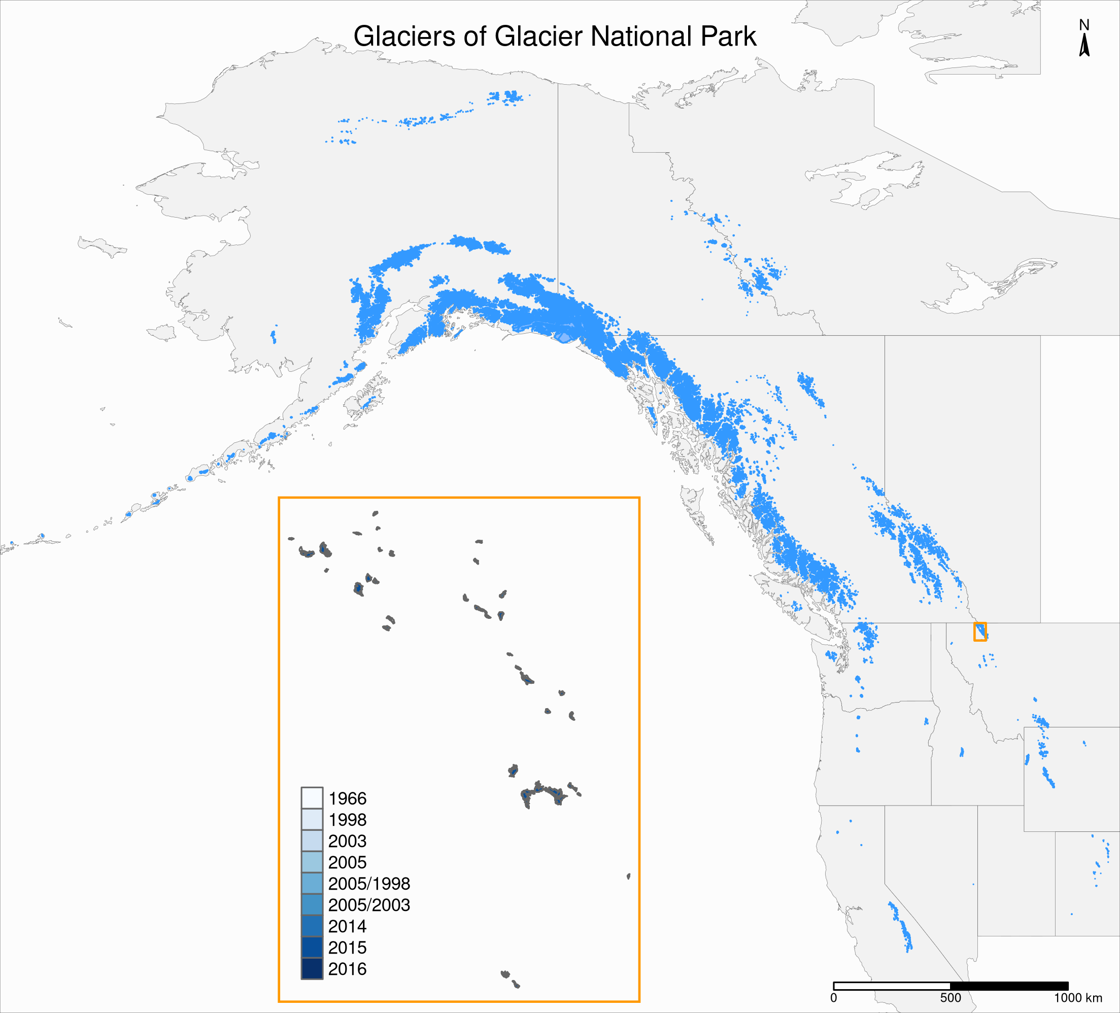
Variation of the inset
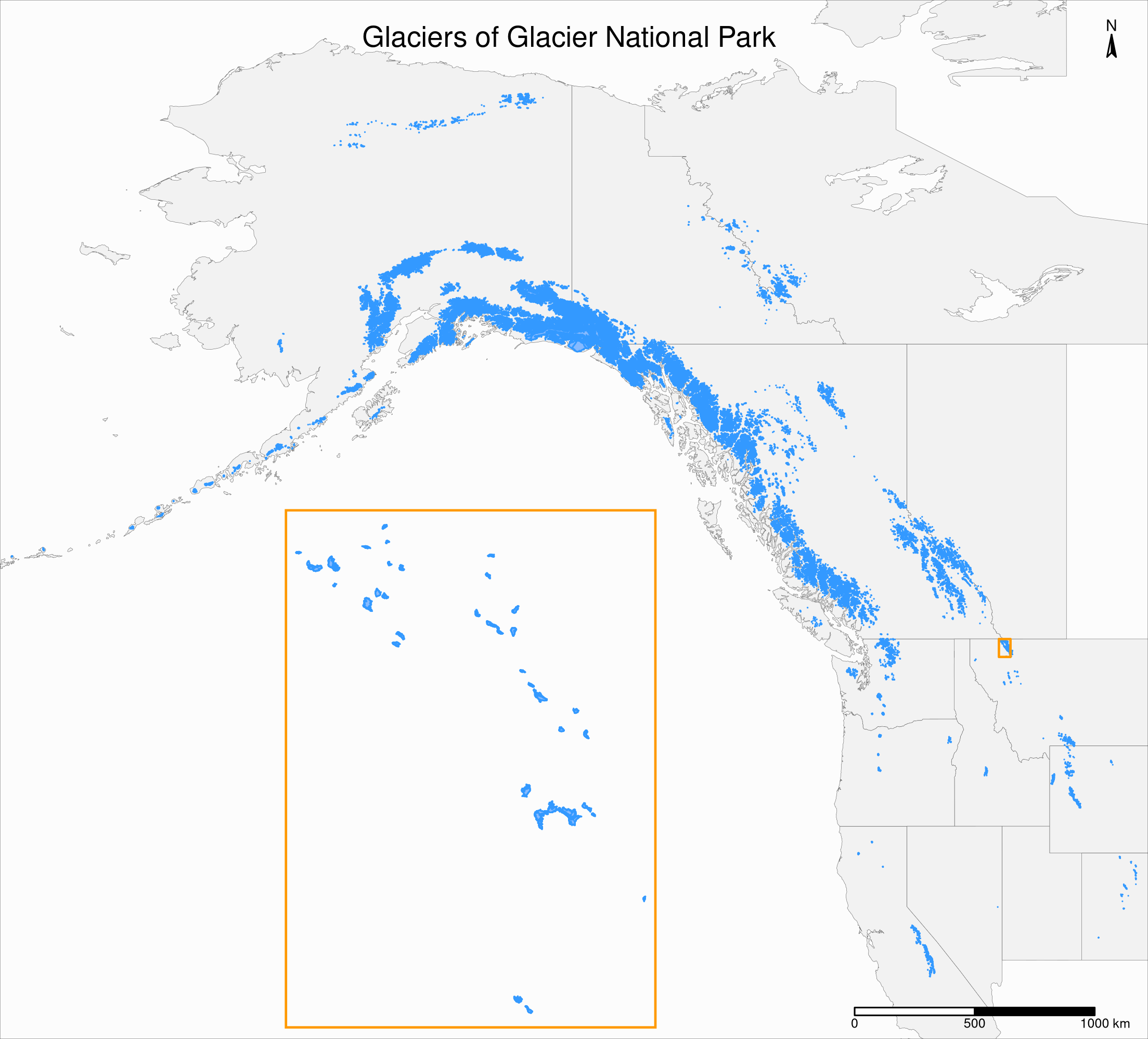
The scale is too small to show the retreat of the glaciers on this map. So it might be better to remove the legend and the palette per year and to make the borders and fill of the same colors as in the main map instead:
inset_map <- tm_shape(gnp) +
  tm_borders(col = "#3399ff") +
  tm_fill(col = "#86baff") +
  tm_layout(
	legend.show = F,
	bg.color = "#fcfcfc",
	inner.margins = c(0.03, 0.03, 0.03, 0.03),
	outer.margins = 0,
	frame = "#ff9900",
	frame.lwd = 3
  )
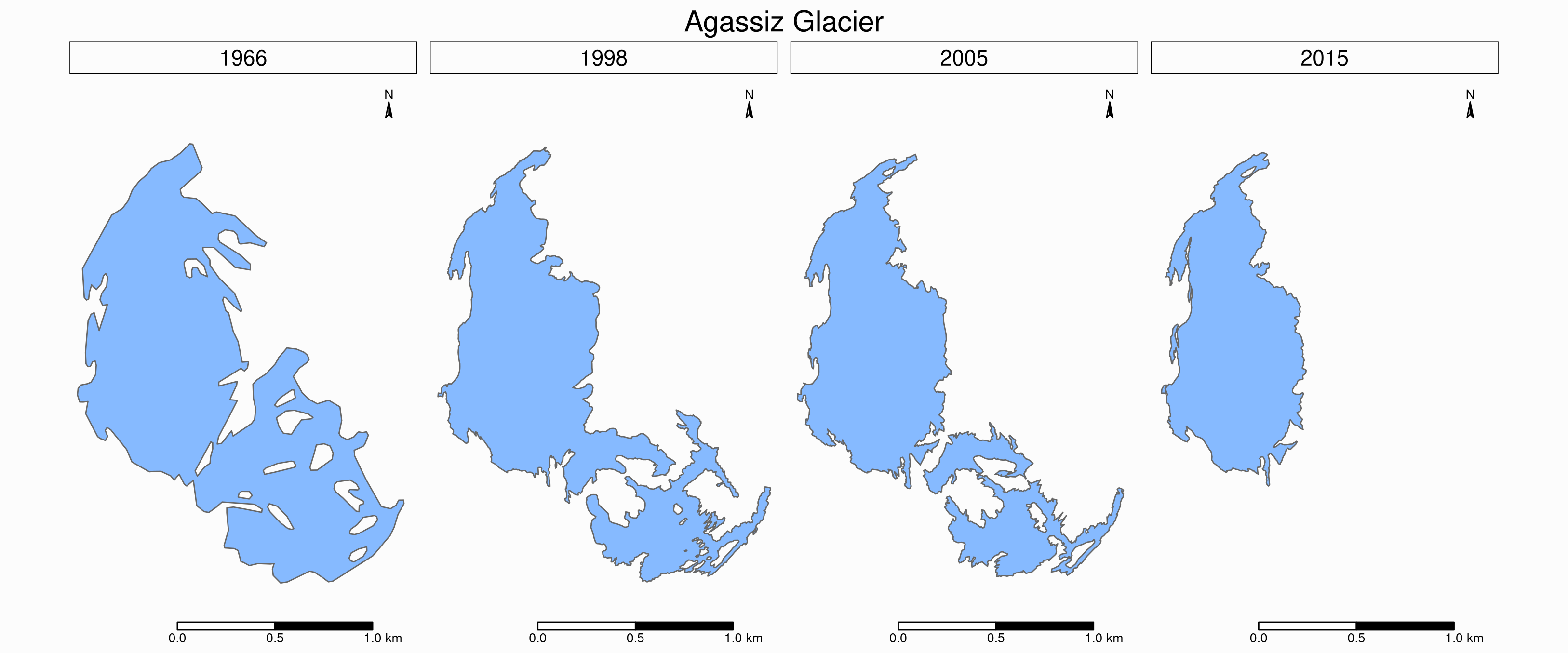
Mapping a subset of the data
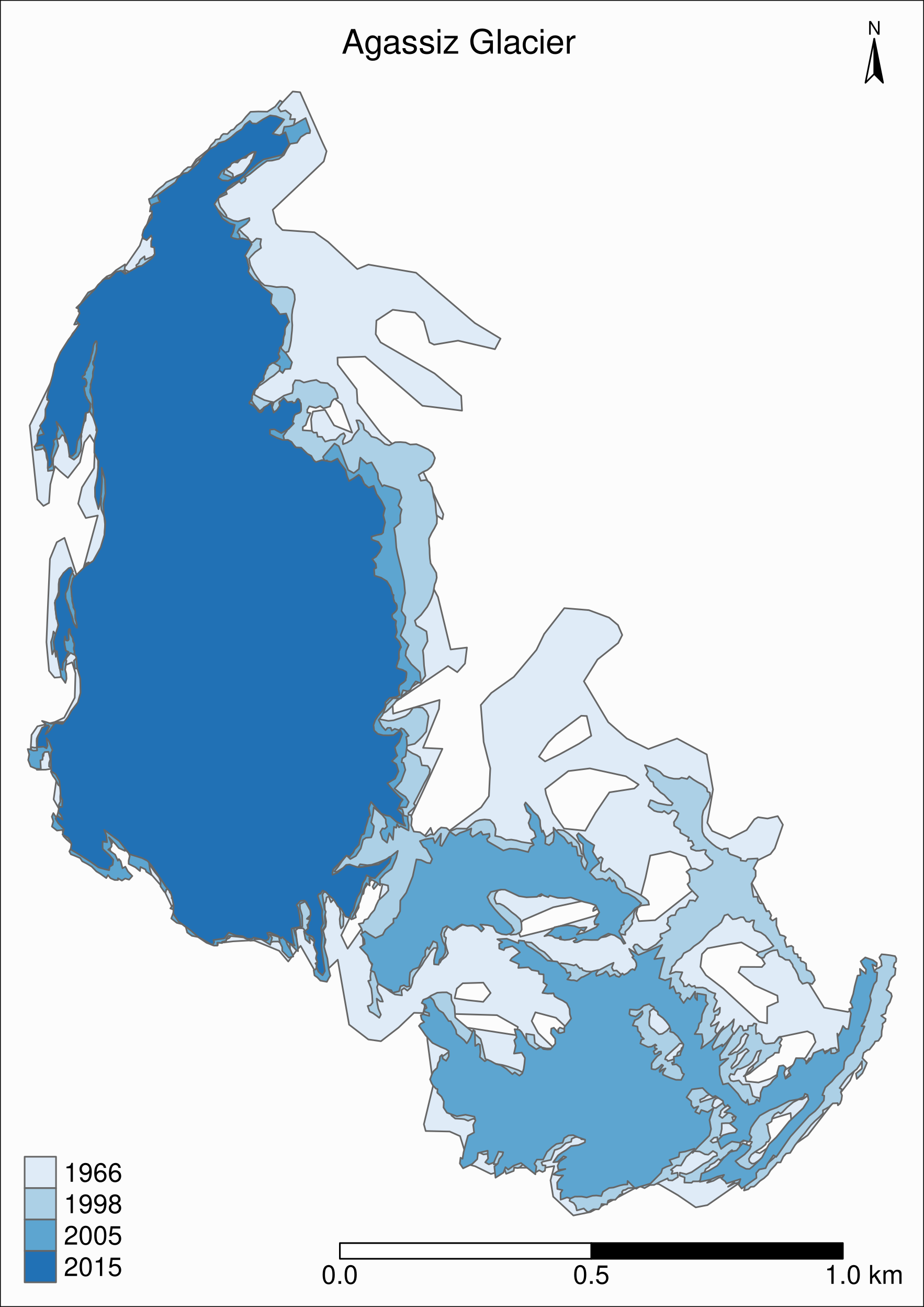
To see the retreat of the glaciers, we need to zoom in on this map. So let’s focus on a single glacier: the Agassiz Glacier.
Map of the Agassiz Glacier
Select the data points corresponding to the Agassiz Glacier:
ag <- g %>% filter(glacname == "Agassiz Glacier")Map of the Agassiz Glacier
tm_shape(ag) +
  tm_polygons("year", palette = "Blues") +
  tm_layout(
	title = "Agassiz Glacier",
	title.position = c("center", "top"),
	legend.position = c("left", "bottom"),
	legend.title.color = "#fcfcfc",
	legend.text.size = 1,
	bg.color = "#fcfcfc",
	inner.margins = c(0.07, 0.03, 0.07, 0.03),
	outer.margins = 0
  ) +
  tm_compass(
	type = "arrow",
	position = c("right", "top"),
	text.size = 0.7
  ) +
  tm_scale_bar(
	breaks = c(0, 0.5, 1),
	position = c("right", "BOTTOM"),
	text.size = 1
  )
Using ggplot2 instead of tmap
As an alternative to the tmap package, ggplot2 can plot maps with the geom_sf() function.
The previous map can be reproduced (with some tweaking of style and layout) with:
ggplot(ag)+
  geom_sf(aes(fill = year)) +
  scale_fill_brewer(palette = "Blues")
Other ways to add a basemap
Basemap with ggmap
basemap <- get_map(
  bbox = c(
	left = st_bbox(ag)[1],
	bottom = st_bbox(ag)[2],
	right = st_bbox(ag)[3],
	top = st_bbox(ag)[4]
  ),
  source = "osm"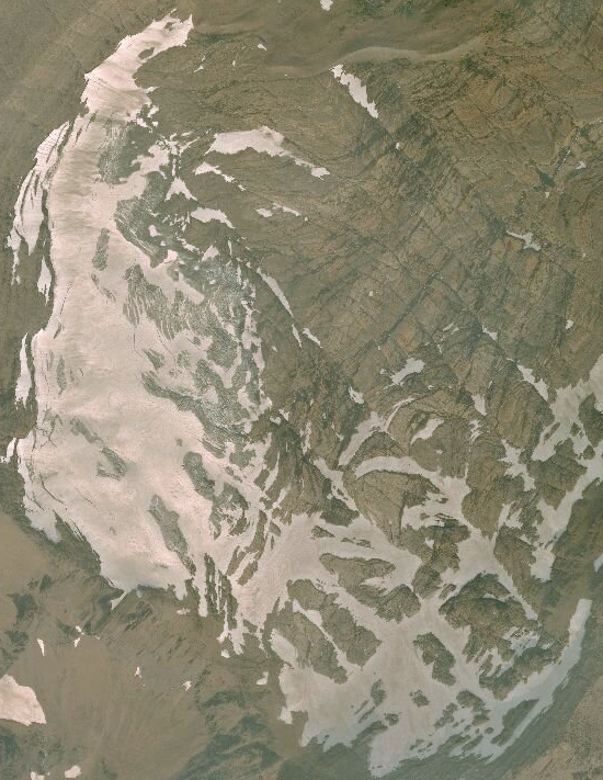
)Basemap with basemaps
The package basemaps allows to download open source basemap data from several sources, but those cannot easily be combined with sf objects.
This plots a satellite image of the Agassiz Glacier:
basemap_plot(ag, map_service = "esri", map_type = "world_imagery")Satellite image of the Agassiz Glacier
Faceted map
Faceted map of the retreat of Agassiz Glacier
tm_shape(ag) +
  tm_polygons(col = "#86baff") +
  tm_layout(
	main.title = "Agassiz Glacier",
	main.title.position = c("center", "top"),
	main.title.size = 1.2,
	legend.position = c("left", "bottom"),
	legend.title.color = "#fcfcfc",
	legend.text.size = 1,
	bg.color = "#fcfcfc",
	## inner.margins = c(0, 0.03, 0, 0.03),
	outer.margins = 0,
	panel.label.bg.color = "#fcfcfc",
	frame = F,
	asp = 0.6
  ) +
  tm_compass(
	type = "arrow",
	position = c("right", "top"),
	size = 1,
	text.size = 0.6
  ) +
  tm_scale_bar(
	breaks = c(0, 0.5, 1),
	position = c("right", "BOTTOM"),
	text.size = 0.6
  ) +
  tm_facets(
	by = "year",
	free.coords = F,
	ncol = 4
  )
Animated map
Animated map of the Retreat of Agassiz Glacier
First, we need to create a tmap object with facets:
agassiz_anim <- tm_shape(ag) +
  tm_borders() +
  tm_fill(col = "#86baff") +
  tm_layout(
	title = "Agassiz Glacier",
	title.position = c("center", "top"),
	legend.position = c("left", "bottom"),
	legend.title.color = "#fcfcfc",
	legend.text.size = 1,
	bg.color = "#fcfcfc",
	inner.margins = c(0.08, 0, 0.08, 0),
	outer.margins = 0
  ) +
  tm_compass(
	type = "arrow",
	position = c("right", "top"),
	text.size = 0.7
  ) +
  tm_scale_bar(
	breaks = c(0, 0.5, 1),
	position = c("right", "BOTTOM"),
	text.size = 1
  ) +
  tm_facets(
	along = "year",
	free.coords = F
  )
Animated map of the Retreat of Agassiz Glacier
Then we can pass that object to tmap_animation():
tmap_animation(
  agassiz_anim,
  filename = "ag.gif",
  dpi = 300,
  inner.margins = c(0.08, 0, 0.08, 0),
  delay = 100
)
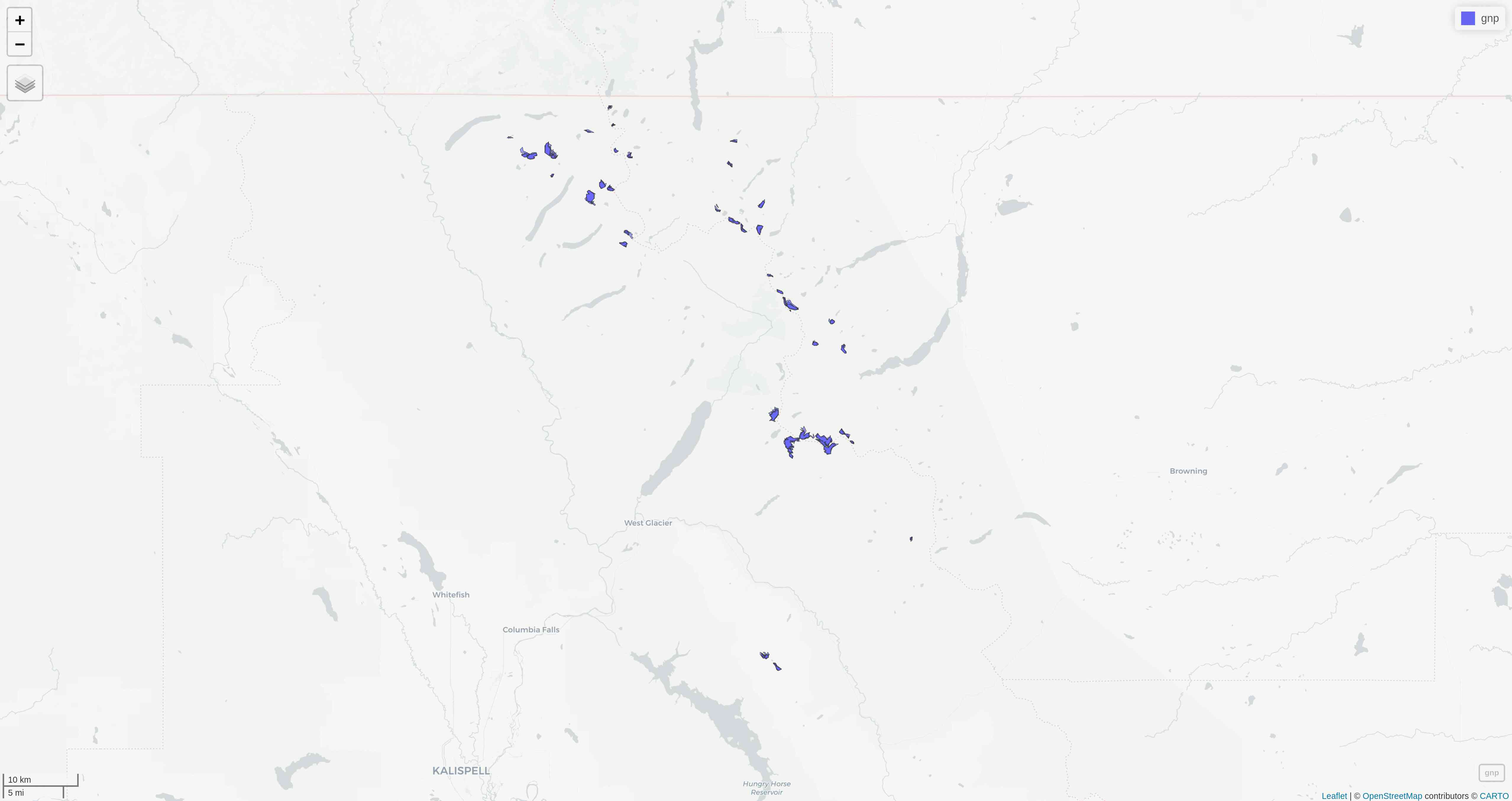
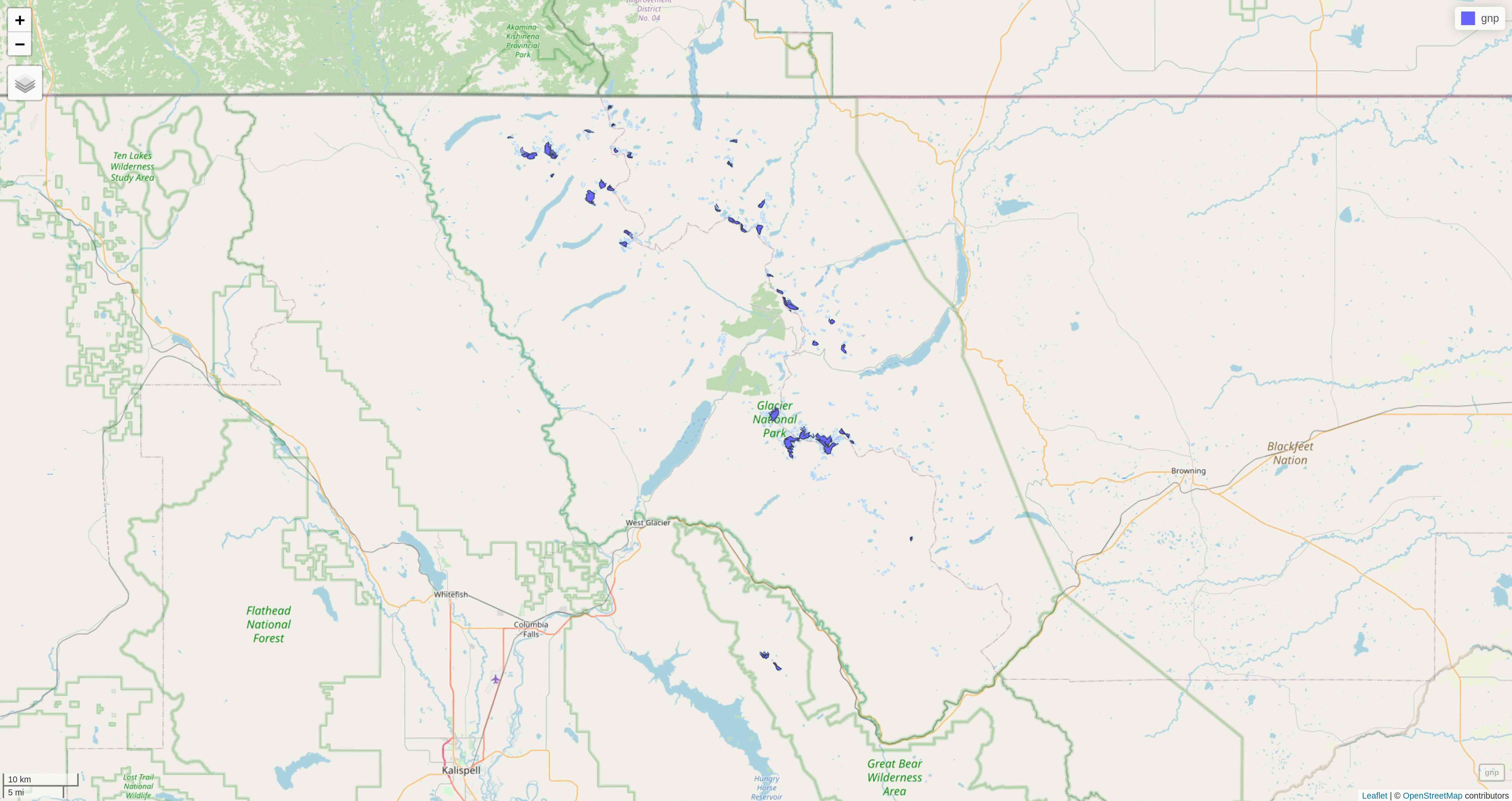
Tiled web maps with Leaflet
Tiled web maps with Leaflet
mapview
mapview(gnp)Tiled web maps with Leaflet
mapview
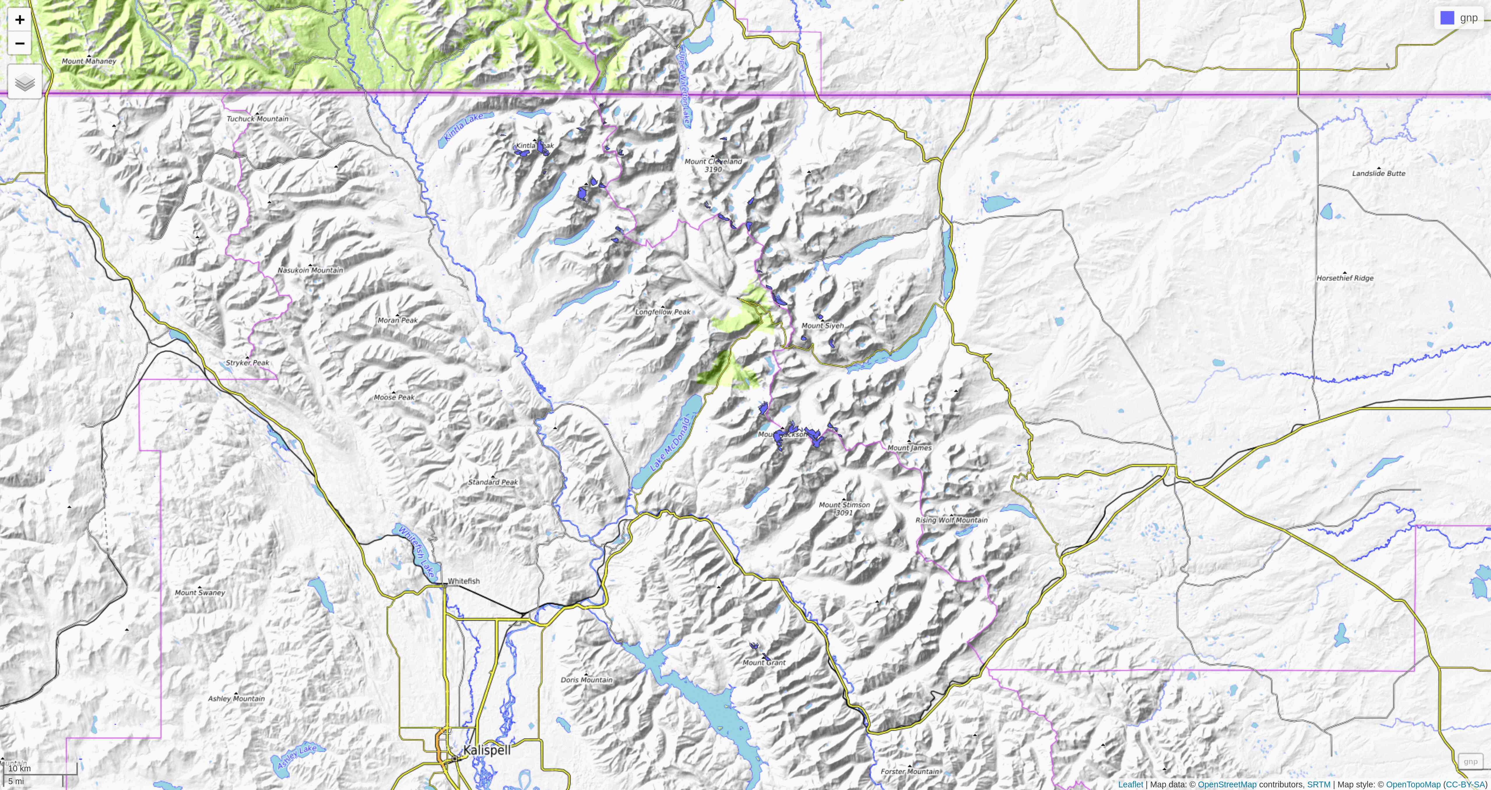
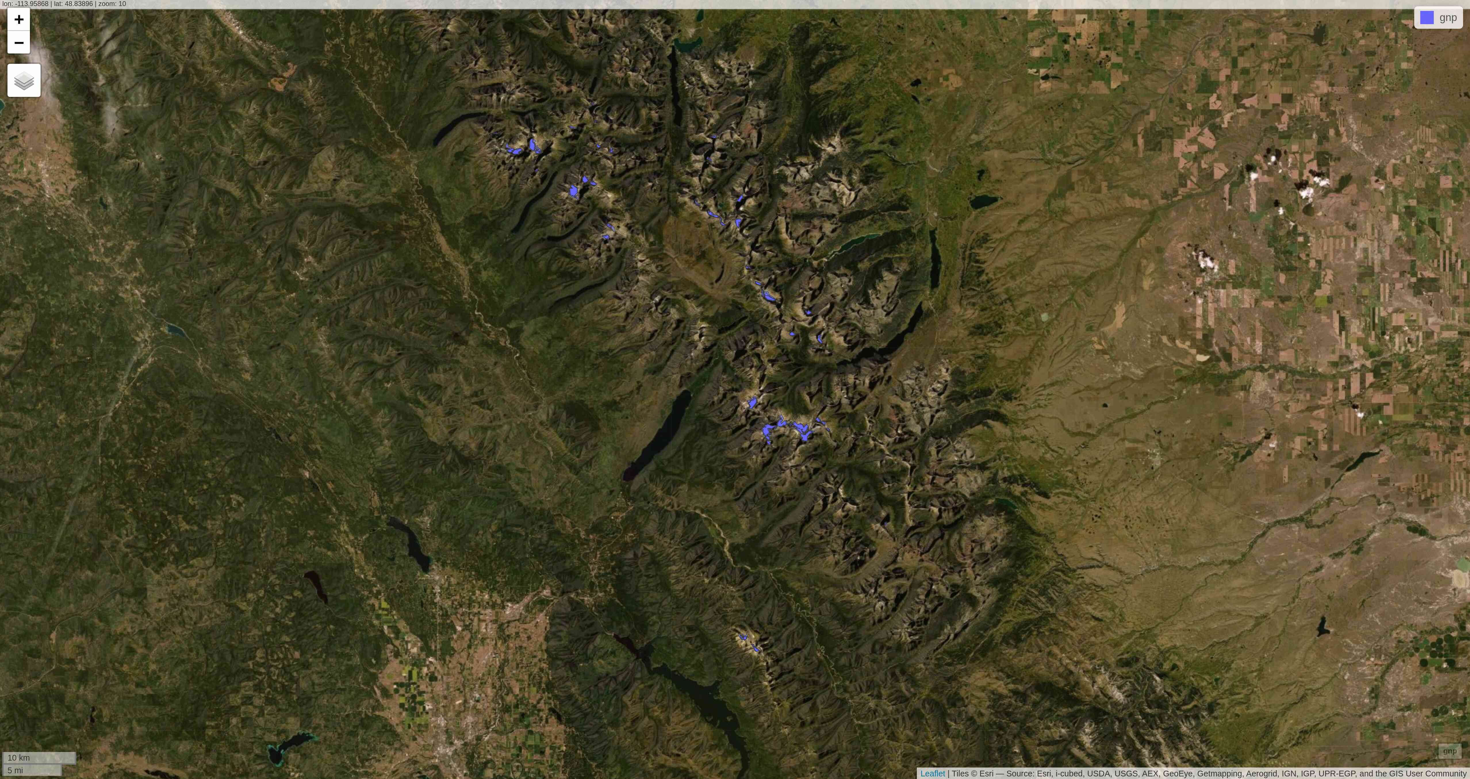
Tiled web maps with Leaflet
tmap
So far, we have used the plot mode of tmap. There is also a view mode which allows interactive viewing in a browser through Leaflet
.
Change to view mode:
tmap_mode("view")Re-plot the last map we plotted with tmap:
tmap_last()Tiled web maps with Leaflet
leaflet
leaflet() creates a map widget to which you add layers.
map <- leaflet()
addTiles(map)
raster
Package for spatial raster (gridded) data
Ice thickness
The nomenclature for glaciers and regions in the ice thickness dataset follows the Randolph Glacier Inventory (RGI) version 6.0.
Let’s look for the Agassiz Glacier data.
RGIId for Agassiz Glacier
> wes %>%
	filter(Name == "Agassiz Glacier MT") %>%
	select(RGIId)
Simple feature collection with 1 feature and 1 field
geometry type:  MULTIPOLYGON
dimension:      XY
bbox:           xmin: -114.1673 ymin: 48.92498 xmax: -114.1442 ymax: 48.94501
geographic CRS: WGS 84
RGIId                       geometry
1 RGI60-02.16664 MULTIPOLYGON (((-114.1487 4...
Now we now which file we need to look for in the ice thickness dataset: RGI60-02.16664_thickness.tif.
Load raster data for Agassiz Glacier
First, we want to see how many bands are available:
> nlayers(stack("RGI60-02/RGI60-02.16664_thickness.tif"))
[1] 1
This is not a multi-layer band (such as an RGB file), so we don’t have to worry about band selection:
agras <- raster("RGI60-02/RGI60-02.16664_thickness.tif")Inspect raster data
> agras
class      : RasterLayer
dimensions : 93, 74, 6882  (nrow, ncol, ncell)
resolution : 25, 25  (x, y)
extent     : 707362.5, 709212.5, 5422962, 5425288  (xmin, xmax, ymin, ymax)
crs        : +proj=utm +zone=11 +datum=WGS84 +units=m +no_defs
source     : /RGI60-02/RGI60-02.16664_thickness.tif
names      : RGI60.02.16664_thickness
Inspect raster data
> str(agras)
Formal class 'RasterLayer' [package "raster"] with 12 slots
..@ file :Formal class '.RasterFile' [package "raster"] with 13 slots
.. .. ..@ name : chr "RGI60-02/RGI60-02.16664_thickness.tif"
.. .. ..@ datanotation: chr "FLT4S"
.. .. ..@ byteorder : chr "little"
.. .. ..@ nodatavalue : num -Inf
.. .. ..@ NAchanged : logi FALSE
.. .. ..@ nbands : int 1
.. .. ..@ bandorder : chr "BIL"
.. .. ..@ offset : int 0
.. .. ..@ toptobottom : logi TRUE
.. .. ..@ blockrows : int 27
.. .. ..@ blockcols : int 74
.. .. ..@ driver : chr "gdal"
.. .. ..@ open : logi FALSE
..@ data :Formal class '.SingleLayerData' [package "raster"] with 13 slots
.. .. ..@ values : logi(0)
.. .. ..@ offset : num 0
.. .. ..@ gain : num 1
.. .. ..@ inmemory : logi FALSE
.. .. ..@ fromdisk : logi TRUE
.. .. ..@ isfactor : logi FALSE
.. .. ..@ attributes: list()
.. .. ..@ haveminmax: logi FALSE
.. .. ..@ min : num Inf
.. .. ..@ max : num -Inf
.. .. ..@ band : int 1
.. .. ..@ unit : chr ""
.. .. ..@ names : chr "RGI60.02.16664_thickness"
..@ legend :Formal class '.RasterLegend' [package "raster"] with 5 slots
.. .. ..@ type : chr(0)
.. .. ..@ values : logi(0)
.. .. ..@ color : logi(0)
.. .. ..@ names : logi(0)
.. .. ..@ colortable: logi(0)
..@ title : chr(0)
..@ extent :Formal class 'Extent' [package "raster"] with 4 slots
.. .. ..@ xmin: num 707362
.. .. ..@ xmax: num 709212
.. .. ..@ ymin: num 5422962
.. .. ..@ ymax: num 5425288
..@ rotated : logi FALSE
..@ rotation:Formal class '.Rotation' [package "raster"] with 2 slots
.. .. ..@ geotrans: num(0)
.. .. ..@ transfun:function ()
..@ ncols : int 74
..@ nrows : int 93
..@ crs :Formal class 'CRS' [package "sp"] with 1 slot
.. .. ..@ projargs: chr "+proj=utm +zone=11 +datum=WGS84 +units=m +no_defs"
..@ history : list()
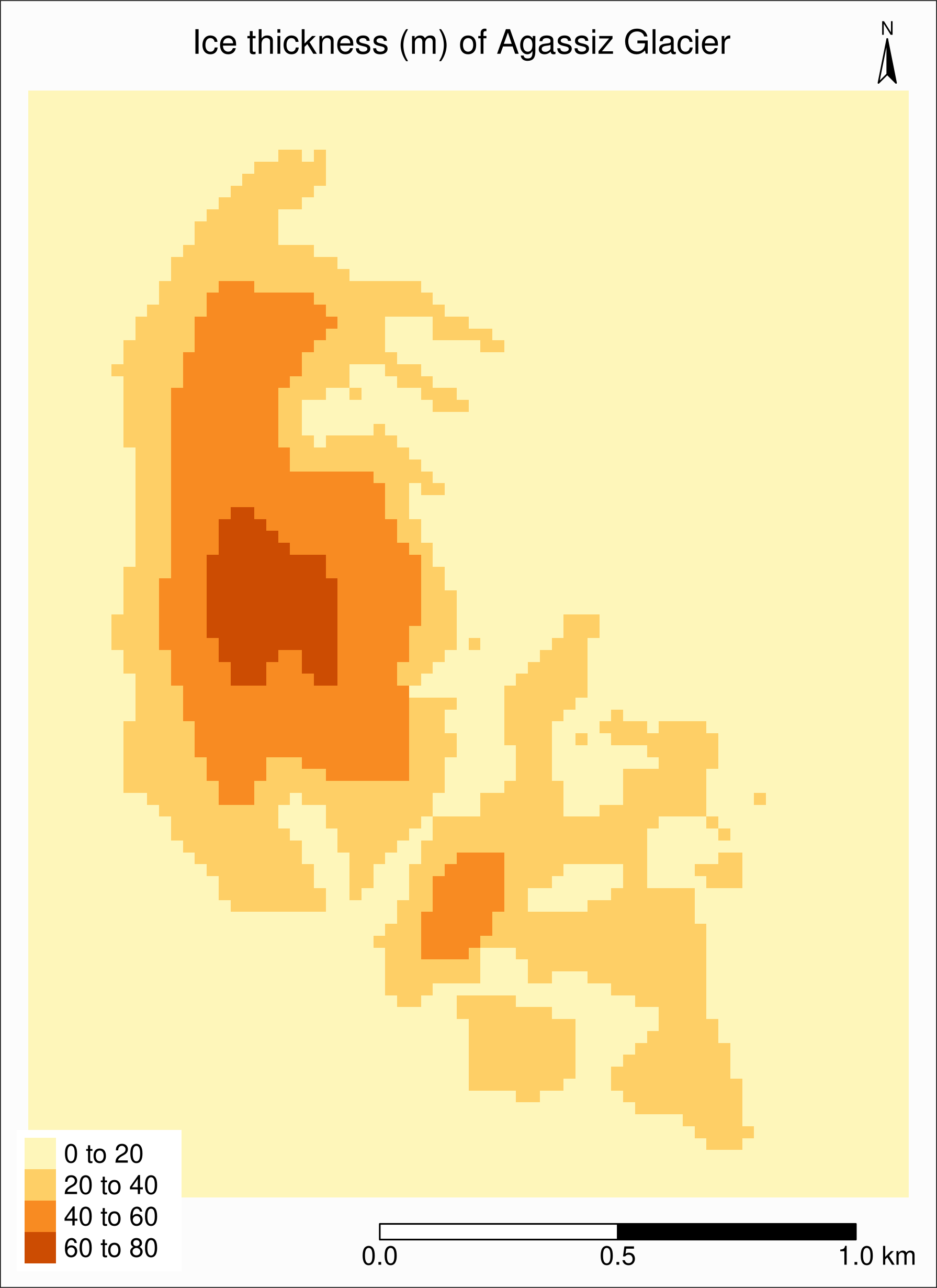
..@ z : list()Map of ice thickness Agassiz Glacier
This time, we use tm_raster():
tm_shape(agras) +
  tm_raster() +
  tm_layout(
	title = "Ice thickness (m) of Agassiz Glacier",
	title.position = c("center", "top"),
	legend.position = c("left", "bottom"),
	legend.bg.color = "#d9d9d9",
	legend.title.color = "#d9d9d9",
	legend.text.size = 1,
	bg.color = "#fcfcfc",
	inner.margins = c(0.07, 0.03, 0.07, 0.03),
	outer.margins = 0
  ) +
  tm_compass(
	type = "arrow",
	position = c("right", "top"),
	text.size = 0.7
  ) +
  tm_scale_bar(
	breaks = c(0, 0.5, 1),
	position = c("right", "BOTTOM"),
	text.size = 1
  )
Combining with Randolph data
As always, we check whether the CRS are the same:
> st_crs(ag) == st_crs(agras)
[1] FALSE
We need to reproject ag (easier than reprojecting the raster object):
ag %<>% st_transform(st_crs(agras))We can verify that the CRS of both our maps are now the same:
> st_crs(ag) == st_crs(agras)
[1] TRUE
Combining with Randolph data
The retreat and ice thickness layers will hide each other (the order matters!).
One option is to use tm_borders() only for one of them, or we can use transparency (alpha):
tm_shape(agras) +
  tm_raster() +
  tm_shape(ag) +
  tm_polygons("year", palette = "Blues", alpha = 0.2) +
  tm_layout(
	title = "Ice thickness (m) and retreat of Agassiz Glacier",
	title.position = c("center", "top"),
	legend.position = c("left", "bottom"),
	legend.bg.color = "#e6e6e6",
	legend.title.color = "#e6e6e6",
	legend.text.size = 0.7,
	bg.color = "#fcfcfc",
	inner.margins = c(0.07, 0.03, 0.07, 0.03),
	outer.margins = 0
  ) +
  tm_compass(
	type = "arrow",
	position = c("right", "top"),
	text.size = 0.7
  ) +
  tm_scale_bar(
	breaks = c(0, 0.5, 1),
	position = c("right", "BOTTOM"),
	text.size = 1
  )